

George Rebane
Here’s a little something from my financial engineering toy box that one or two RR readers may find interesting. The discussion is a tiny bit technical, but the pictures should be accessible to all. Most investors know that a stock’s beta (Greek β) is a number that indicates how well the security tracks its market, say, the SP500. And rho (Greek ρ) measures the correlation between, say, the price series of two stock’s – the way they both zig and zag together, or how much one zigs while the other zags. I’ll try to keep this short.
From august sources like Modern Portfolio Theory (MPT) by nobelists Markowitz and Sharpe, we learn that if a stock’s β equals one, then it more or less goes up and down in similar percent changes with the market. If β > 1, then the stock’s swings have a greater percentage than the market’s; and if β < 1, then the stock’s swings behave in a more reserved manner than do the market’s. Riskier stocks have the bigger swings, and more conservative stocks have the smaller swings. The referenced formula (here) for beta reflects this with its inclusion of the standard deviation of the price swings.
As stated above, ρ measures in how tight of a formation two stocks will fly. The range of ρ is between +1 and -1, with the positive values indicating tighter formations, and ρ = 1 denoting a perfectly tight formation matching each other’s zigs and zags. A small or zero ρ means that the stocks pretty much act independently of each other. In designing your investment portfolio from a selected shortlist of stocks, MPT teaches that you should try to avoid stocks that pair with high ρ values. Doing probabilistic math recommends that you pick stocks that pair with the lowest ρ values possible to give you a low volatility (i.e. low risk) portfolio.
Now after you understand all that, we’re going to throw a monkey wrench into the whole thing, a little bit of information you will not hear from your well-paid wealth advisor who manages your portfolio. (Drum roll please.) Betas and rhos, calculated from past performance, are pretty much worthless measures of securities performance for portfolio design. Why? Well, that answer depends on what is known as the investor’s ‘investment horizon’. That’s the period into the future over which the investment plan is supposed to hold with numbers such as expected portfolio appreciation, its most likely upper and lower limits, and so forth.
Securities traders come mostly in three flavors of investment horizons – short range or day traders (1-5 days), range traders (few months to a year), and long-term traders (multiple years). Rebanes are range traders and look at 6 – 12 month investment horizons for the securities we hold. Now that doesn’t mean that we turn over our entire portfolio every year; it just means that we re-evaluate the stocks within that investment horizon.
But here’s the big fallacy in using the rhos and betas over any extended investment horizon – they don’t remain constant and vary all over the place. No matter what values you pick for them, they are guaranteed to change significantly over the next several months to years. And portfolio theories such as MPT all assume that beta and rho stay put with their assigned values to the end of your investment horizon. And here’s another little wiggle in using such critical parameters for your investment decisions – both rho and beta are almost always derived from past price histories over chosen time intervals, usually the last couple of quarters or year.
But there’s no guarantee the financial environment (markets, business prospects, monetary and fiscal policies) will remain unchanged over the next such periods. In fact, I can guarantee that they won’t. So, the calculated values of beta and rho are pretty much fiction (‘brown numbers’) in their use as constants for portfolio design. (An interesting anecdote is that it is almost impossible to find an investment professional who uses MPT to design their own portfolios. But they have no problem using it to fashion yours for a handsome fee. Why? Because it’s the best CYA for the investment advisor in the event you decide to sue because your portfolio tanked – ‘Hey, I used MPT with two Nobel prizes under its belt, doesn’t everyone?’
If you’re still with me, you get to look at some pretty pictures of how rho and beta misbehave. I downloaded about ten years of closing price data for the SP500, AAPL (Apple), EOS (high yield income ETF), and XLE (ETF of energy stocks). Then I wrote some code that allowed me to compute the rhos and betas from selectable past time windows, and also compare these over future time horizons. A sample of the outputs are presented for your edification and enjoyment.
The first plot below shows the correlation coefficient rho between AAPL and XLE over a trailing 125 trading-day window that is computed as a rolling value over a period of about ten years. It is clear that these two seemingly independent securities vary as much as possible with the passing of the years. Take any trailing window to compute a prediction of rho over a future investment horizon, and you will see a markedly different rho value that obtains over this future time interval. So, what pairwise rho values are you going to use to select your shortlist of stocks? (For those with investment advisors, show them this plot and give them a link to this post. At a minimum, their response should be entertaining.)

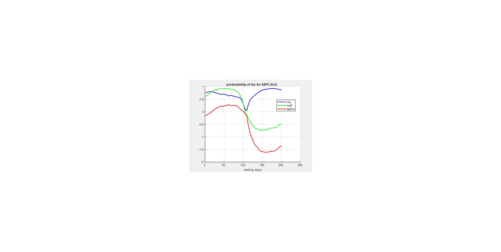
Finally, to drive home the point of this expose, we take a look at the predictability of rho over a short 200 trading day window (here from trading 600 to 800). The figure below shows in blue the behavior of rho, calculated from the last 125 trading days, in that interval. Similarly, in green we see rhoF, the actual future value of rho calculated over the next 125 trading days. The difference between the two is shown in red, and ideally we would like to see this line hover around zero, indicating that our calculated rho would serve well to predict its future value. However, the red trace shows that blatantly this is not the case, substantiating our thesis that using past time series to predict the correlation behavior of two stocks ranges from pretty much useless to possibly harmful to your portfolio’s performance.

It’s important to note here that such results can be seen for any two securities over literally any sliding window of trading days. This effect underlines the usual cautionary ‘past performance is not a guarantee of future results’. So how should we derive rho values for our shortlist of stocks, if not from past data? Well, unfortunately the answer is that such an estimate of rhoF should come from the investor’s own apprehension of economic prospects for the pair over his investment horizon. This process is of necessity highly personalized, and will involve considering many factors depending on the investor’s acumen. And what about beta in view of the above? Since the formula for beta involves rho as a multiplicative factor, then to the extent that rhoF is bogus, so is betaF. A more detailed discussion of developing rho and beta values is out of scope for what has been presented. (Technically, this involves different methodologies for calculating the covariance matrix for the shortlist of stocks as required by most portfolio design models.)
[Addendum] Asset (e.g. stocks) price performance prediction models and portfolio (composed of such assets) design models are distinct instruments yielding different information sets to the investor. The above discussion addressed two common asset performance parameters, calculated from past price histories and often used to predict future assets’ performance. I emphasize ‘asset’ here because rho and beta can be computed for any asset whose market price history is available – e.g. numismatic coins, real estate, commodity contracts, the oeuvre of a rock star, … .
Almost all portfolio design models permit the use of a variety of performance prediction models to obtain the necessary asset price predictions over the investment horizon. The minimal requirements from the prediction models are the expected prices and covariance of the assets in the portfolio designers shortlist of assets. For example, MPT the expected prices and the covariance matrix of the shortlist assets at the investment horizon. From this can be computed its required expected returns and normalized variances and covariances.
Like most design models, MPT then searches the asset-weights space to find the optimum weight or allocation vector for the shortlist assets. MPT actually finds an ‘infinite set’ of optimum portfolio weights which it characterizes in the form of a curve known as the efficient frontier drawn so that the x-axis represents the standard deviation of price variability (MPT’s risk/volatility parameter), and the y-axis represents the expected portfolio return at a given weight vector or allocation fractions. The efficient frontier is made of points that vary the weight vector to yield the minimum sigma (i.e. risk) at a given value of expected return. (Here is a good MPT reference with appropriate graphics.) MPT then defines the single best portfolio that balances return and risk at the point where the so-called ‘capital allocation line’, starting on the y-axis at the current ‘risk-free rate’ (e.g. US Treasuries), just grazes the efficient frontier.
One of the many problems with MPT is that, starting with the same shortlist of assets, the best allocation vector for both you and Jeff Bezos or Elon Musk or … is exactly the same. And everyone knows that is not true, since the tolerance for monetary risk varies widely, depending on your current net assets among other factors. A useful alternative for such portfolio design tools are those that take investors’ monetary utility into account. These then can provide individualized portfolio designs instead of one-size-fits-all portfolios that MPT computes.
At this point it is important to recall that any given portfolio design method will yield different results that depend not only on what asset prediction models are used, but also on the specific parameter values (representing the investor’s beliefs) used in any such model. Complex stuff with a lot of dependers, all of which emphasizes that there is no free lunch.

Leave a comment